Section 1 Function gallery
Subsection 1.1 Prototypical examples of bidegree \((1, n)\) RISPs
Example 1.1. A favorite function.
Consider the function \(\Phi\) given by
This function and basic variants are the foundational example in the study of rational inner functions in two variables.
Example 1.3. Agler, McCarthy, Young function.
Consider the rational inner function
which features as an example in the paper [3.3], and has been further studied in [3.9][Section 1.3] and [3.6][Example 5.2] (without the minus sign in front).
The corresponding RISP \(\Phi(z,w) = (\phi, w)\) has a SF point corresponding to a normal crossing of invariant components and a rotation band.
Subsection 1.2 \((1, n)\) RISPs with more complex behavior
Example 1.5. Stacked rotation belts.
Consider the function
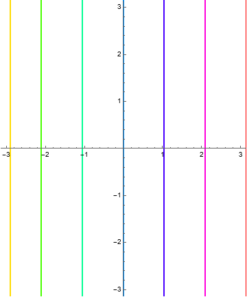
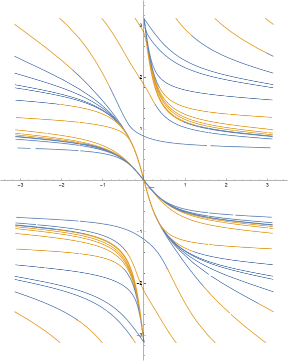
The invariant curves and level curves are
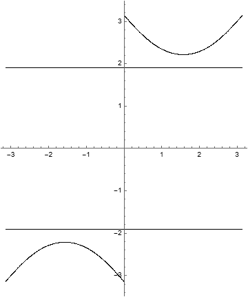
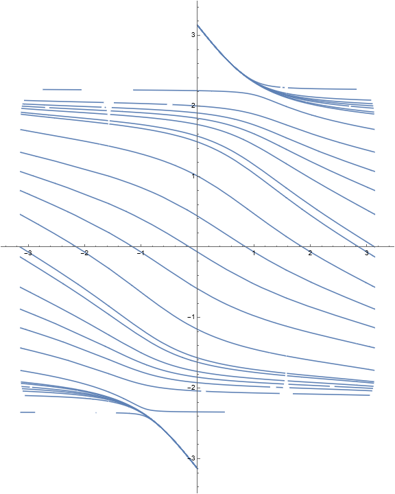
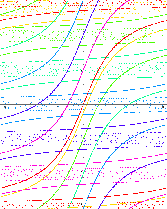
The dynamical behavior for several iterations of \(\Phi\) is 
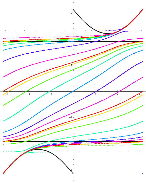
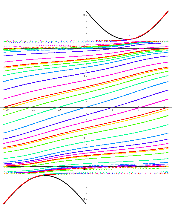
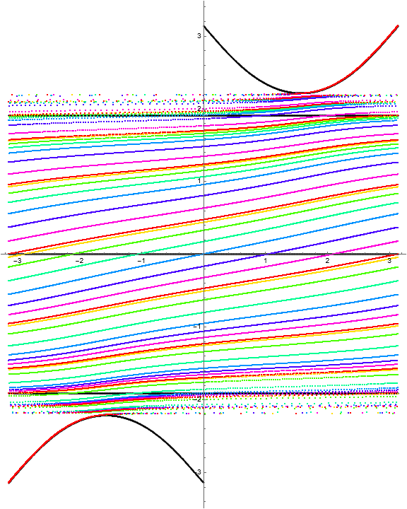
Because there are three horizontal invariant curves, we should observe four “stacked” rotation belts bounded by identity fiber maps. A computation of the multipliers as a function of \(w\) gives the following visualization. 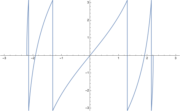
Example 1.10. Multiple crossings.
Consider the function
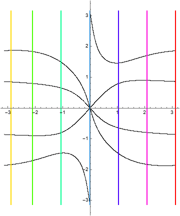
The invariant curves and level curves are
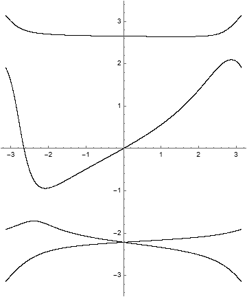
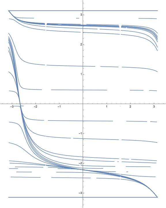
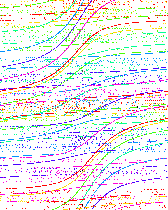
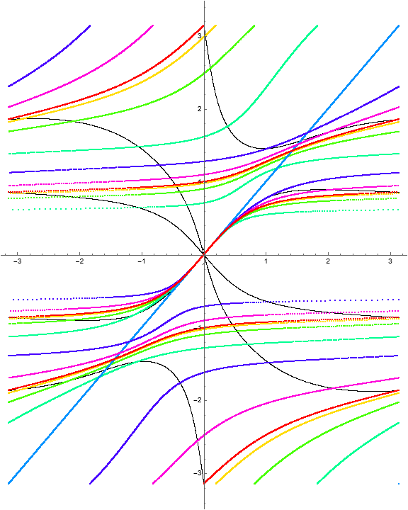
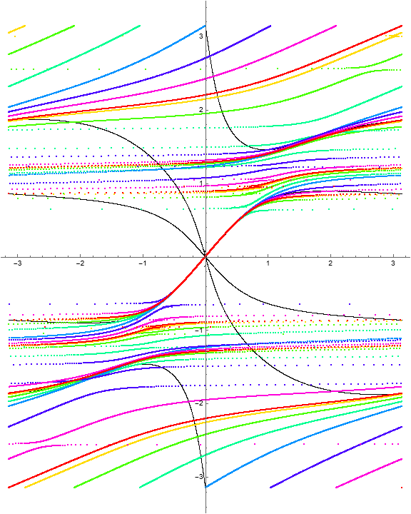
The dynamical behavior for several iterations of \(\Phi\) is 
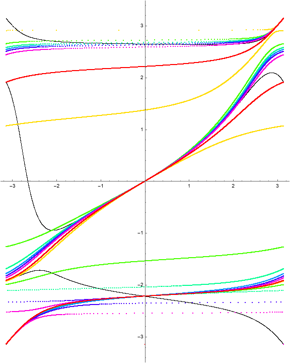
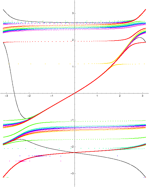
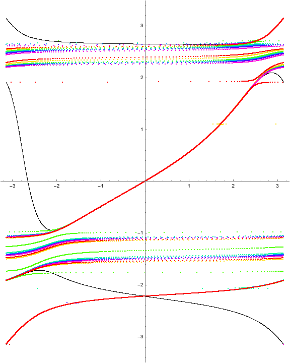
With a choice of \(a = Pi\text{,}\) the polynomial \(Q_a\) factors as
exhibiting the normal crossings visible in the images.
Subsection 1.3 Higher order RISPs
Example 1.14. A degree \((2, 4)\) RISP.
Consider the function given by
which has bidegree \((2, 4)\) as a RISP.
Unlike the \((1, n)\) case, invariant curves can now sweep through rotating fibers.
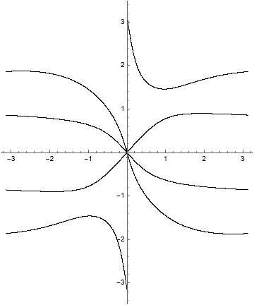
One detail to note in the iteration portraits below is that the rotations are constrained by the fixed point structure of the initial vertical lines.
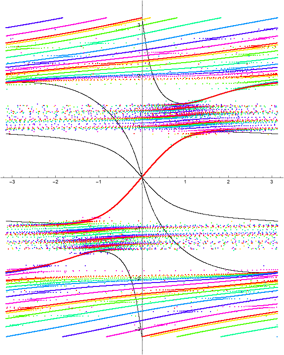
Example 1.18. RISP with \(\Phi = (\phi, w^2)\).
Consider the function \(\Phi\) with
where we have \(\phi_2(w) = w^2\) in the second slot.
Even in this simple case, the behavior of \(\Phi\) is quite different from the related Example 1.1. 
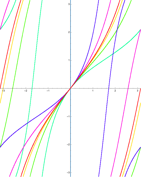
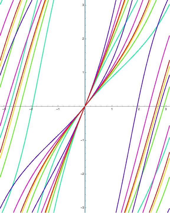
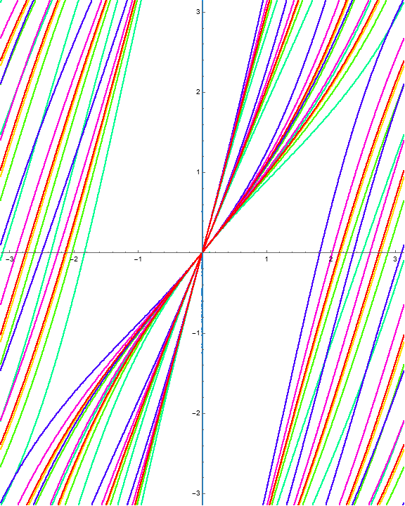
Example 1.20. RISP with \(\Phi = (\phi, i w)\).
Consider the function \(\Phi\) with
where we have \(\phi_2(w) = i w\) in the second slot.
Again, the behavior of \(\Phi\) is quite different from the related Example 1.1. 
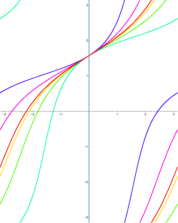
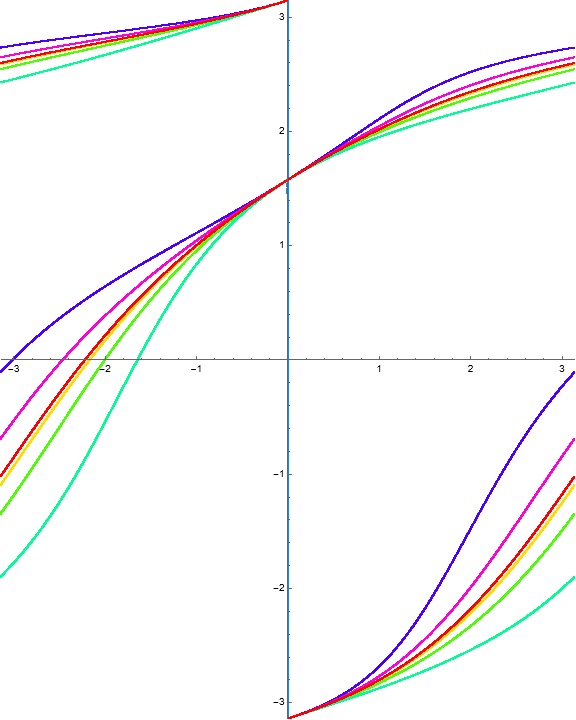
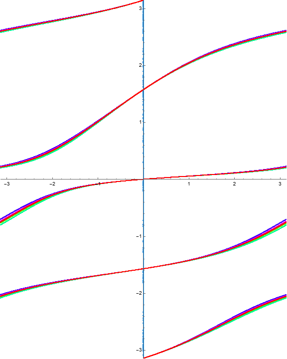
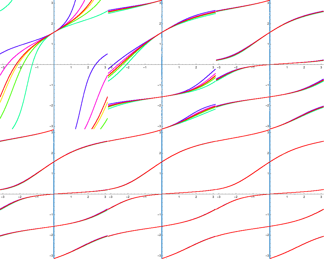
We can observe the periodic structure of the mapping via an animation, where each frame represents the image of that iteration.
Subsection 1.4 Other two-variable examples
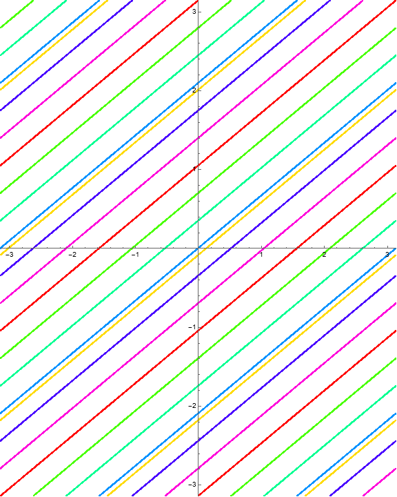
Example 1.23. Monomial mapping.
Consider the function



Example 1.25. Two variable Blaschke products.
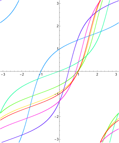
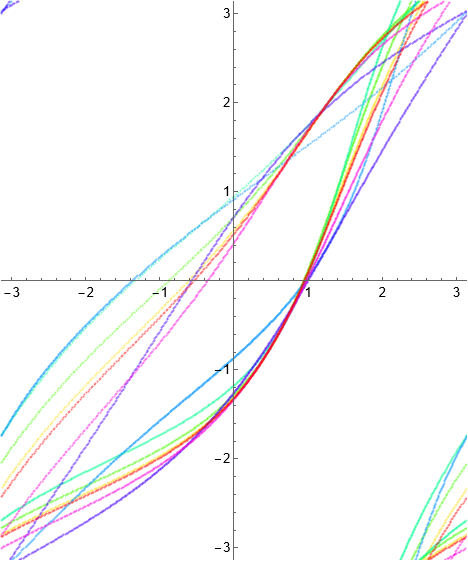
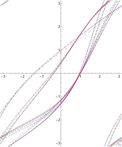
Let
Let \(\Phi\) be the RIM given by
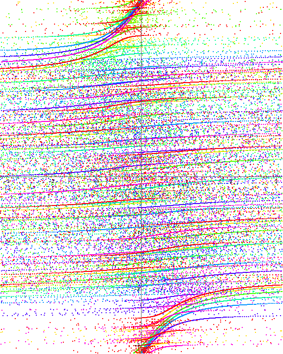
Here, unlike the \((1, n)\) RISP case, we see chaotic behavior. In particular, we do not get curves of fixed points. The dynamical behavior for several iterations of \(\Phi\) is 
Example 1.27. Singular inner function.
Consider the function
with a so-called singular inner function in the first slot.
